In the previous blog post What is Computational Physics (Science)?, I ended the post with the following figure

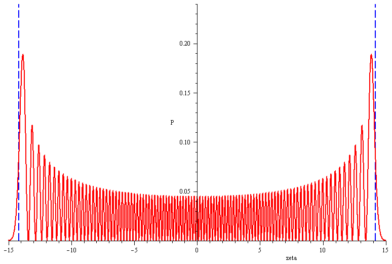
Graph of the probability distribution of the 100th state of the quantum harmonic oscillator (generated using the power series method).

and stated that I might write a post on how to solve the Quantum harmonic oscillator numerically using the power series method (the other method being the ladder operator method [1]) and generate that figure. This post is just about that.

Ok. First I need to clear the cache with the restart command, import the PDEtools (to solve the pde SE) and Maplets[Elements] (necessary if you want to generate a maplet with a slider) packages.

restart;
with(PDEtools): #we need to use the dchange command later in the solution
with(Maplets[Elements]):

I also need to initialize/declare the equations & functions. I assign the Time-Independent Schrodinger Equation (TISE for short) to SE (or whatever variable you wish). Similarly, I assign the potential to V, the allowed energies to E, and the remaining functions & constants to p, q, omega, & lambda:

SE:=(hbar^2/(2*m))*diff(psi(x),x$2)+(E-V)*psi(x)=0:
V:=(1/2)*m*omega^2*x^2:
E:=(n+1/2)*hbar*omega:
p:=zeta->exp(-zeta^2):q:=0:omega:=zeta->exp(-zeta^2):lambda:=2*n:

Now I combine several steps into a single command (which took quite some time to make it work.), which will expand the TISE for V & E (expand), introduce new variables & make variable changes in the TISE (dchange), reexpand the TISE (expand again), solve the new TISE (dsolve), take the right-hand-side of the solution (rhs), convert the solution from a KummerM & KummerU solution to a Hermite solution (convert), remove the KummerM term from the solution for normalization reasons (remove), and finally simplify the result (radsimp):

psi:=(radsimp(remove(has,convert(rhs(dsolve(expand((dchange({x=sqrt(hbar/(m*omega))*zeta,psi(x)=f(zeta)*exp(-zeta^2/2)},(expand(2*SE/(hbar*omega))),[zeta,f(zeta)]))/exp(-zeta^2/2)),f(zeta))),Hermite),KummerM)))*exp(-zeta^2/2);

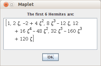
To see the first 6 Hermites, add this code

simplify(HermiteH(0, zeta)), simplify(HermiteH(1, zeta)), simplify(HermiteH(2, zeta)), simplify(HermiteH(3, zeta)), simplify(HermiteH(4, zeta)), simplify(HermiteH(5, zeta))

Or for a maplet

Maplets[Display](Maplet(["The first 6 Hermites are:", MathMLViewer['MMLV1']('value' = [simplify(HermiteH(0, zeta)), simplify(HermiteH(1, zeta)), simplify(HermiteH(2, zeta)), simplify(HermiteH(3, zeta)), simplify(HermiteH(4, zeta)), simplify(HermiteH(5, zeta))]), [Button("OK", Shutdown())]]))

To normalize we need to substitute the value for _C2 which I grabbed from Griffith’s boo (he also borrowed it from another book!), then simplify it with respect to psi & finally write it as an arrow operator [2] using unapply:

P:=unapply(simplify((subs(_C2=sqrt(2^n/(sqrt(Pi)*n!)),psi))^2,exp),n);

To check that normalization is satisfied, I calculate the total probability (i.e over all space, hence -infinity < zeta < infinity) for n=30 (you can choose any value)

Prob:=int(P(30),zeta=-infinity..infinity);

which turns out to be 1, hence the normalization constant _C2 we borrowed from Griffith’s is correct.

One last thing needs to be satisfied; You (not me; I’m not going to write the math here) need to calculate the expression for the operator L; this is done by writing out the “classical” energy conservation equation for the QHO, evaluating v=0 (at the turning points the velocity is zero) & evaluate for zeta. You will get two square roots; the negative one is eliminated & the positive one is assigned to L

L:=n->sqrt(2*n+1):

Finally, we can now make the plot

plot([[[L(100),0],[L(100),0.24]],[[-L(100),0],[-L(100),0.24]],P(100)],zeta=-15..15,numpoints=2000,linestyle=[3,3,1],color=[blue,blue,red],thickness=2,labels=["zeta","P"]);

Here I used 2000 points (numpoints) to plot the curve; you could choose any number you wish. I sued red as a color for the curve & blue for the vertical lines at the turning points.
This will produce the same figure as the one at the beginning of this post. If you look it up in Griffith’s or Gasiorowicz’s book you’ll find it is the same figure except for the vertical axis, which in Maple is centered by default.

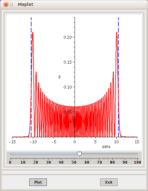
Now to make a maplet like the following one

Maplet with a slider to select a state (between 0 & 100) for the QHO & plot the probability density (P) against position (zeta).

just copy & paste this code to the end of you worksheet (I also copied it from an example from Maple’s documentation & edited it for my needs):

with (Maplets[Elements]):
maplet := 
Maplet('onstartup'='Action1','reference'='Maplet1',
 Action('reference'='clickButton1'),
 Action('reference'='clickButton2',
  Evaluate('function'='plot(TextBox2,zeta = -15 .. 15,numpoints = 2000,linestyle = [3, 3, 1],color = [blue, blue, red],thickness = 2,labels = ["zeta", "P"])','target'='Plotter1','waitforresult'='true')),
 Return('reference'='Return1'),
 Action('reference'='clickButton3',
  Shutdown(`return`='Return1')),
 Plotter('background'="#FFFFFF",'continuous'='true','delay'='100','height'='440','reference'='Plotter1','visible'='true','width'='440'),
 Slider('background'="#D6D3CE",'enabled'='true','filled'='true','foreground'="#000000",'lower'='0','majorticks'='10','minorticks'='1','onchange'='Action7','orientation'='horizontal','reference'='Slider1','showlabels'='true','showticks'='true','snapticks'='true','upper'='100','value'='1','visible'='true'),
 BoxLayout('background'="#D6D3CE",'border'='false','halign'='center','inset'='5','reference'='BoxLayout2','valign'='center','vertical'='false','visible'='true',
  BoxColumn(
   BoxCell('hscroll'='never','value'='Plotter1','vscroll'='never'),
   BoxCell('hscroll'='never','value'='Slider1','vscroll'='never'))),
 TextBox('background'="#FFFFFF",'editable'='false','enabled'='true','foreground'="#000000",'height'='1','reference'='TextBox1','value'="[[[L(n),0],[L(n),0.24]],[[-L(n),0],[-L(n),0.24]],P(n)]",'visible'='false','width'='20','wrapped'='true'),
 TextBox('background'="#FFFFFF",'editable'='false','enabled'='true','foreground'="#000000",'height'='1','reference'='TextBox2','visible'='false','width'='20','wrapped'='true'),
 Button('background'="#D6D3CE",'caption'="Plot",'enabled'='true','foreground'="#000000",'onclick'='clickButton2','reference'='Button2','visible'='true'),
 Button('background'="#D6D3CE",'caption'="Exit",'enabled'='true','foreground'="#000000",'onclick'='clickButton3','reference'='Button3','visible'='true'),
 BoxLayout('background'="#D6D3CE",'border'='false','halign'='center','inset'='5','reference'='BoxLayout1','valign'='center','vertical'='true','visible'='true',
  BoxRow(
   BoxCell('hscroll'='never','value'='BoxLayout2','vscroll'='never')),
  BoxRow(
   BoxCell('hscroll'='never','value'='TextBox1','vscroll'='never'),
   BoxCell('hscroll'='never','value'='TextBox2','vscroll'='never')),
  BoxRow(
   BoxColumn(
    BoxCell('hscroll'='never','value'='Button2','vscroll'='never')),
   BoxColumn(
    BoxCell('hscroll'='never','value'='Button3','vscroll'='never')))),
 Window('layout'='BoxLayout1','reference'='Window1','resizable'='true','title'="Maplet"),
 Action('reference'='Action1',
  RunWindow('window'='Window1')),
 Action('reference'='Action7',
  Evaluate('function'='subs(('n') = ('Slider1'),'TextBox1')','target'='TextBox2','waitforresult'='true'))):

Maplets[Display](maplet);

Here you have it; the analytical (power series) solution for the Quantum harmonic oscillator using Maple. And all this is two-, not three- dimensional!

It is worth noting, as the wikipedia article notes that the QHO is

“…one of the few quantum-mechanical systems for which an exact, analytical solution is known.”

[1] Quantum Harmonic Oscillator -Ladder operator method
[2] Arrow Operator (Maple)